Introduction to Regress Pro
Overview
Regress Pro is an application for the analysis of spectroscopic ellipsometry and reflectometry data.
The application can load spectroscopic data coming from ellipsometers and reflectometers and treat them using well-known fit algorithms to determine physical parameters like film’s thicknesses or their refractive index. The application assume that the data are acquired in reflection mode with an opaque substrate and the spectra are expected to be resolved in the wavelength domain. In the chapter about loading spectra more details are given about what kind of files are accepted by the application.
Using the Application
The first things to do when working with data is to setup a model of the film stack. In the film stack one defines:
- the substrate
- a number of thin films, possibly a single film or none
- the environment where measurement is done.
Each material used in the film stack will be associated to a refractive index resolved in wavelength. In the film stack the thickness of each layer is entered in the corresponding text field on the right. In Regress Pro all the thicknesses are expressed in Angstrom and the wavelengths in nanometers.
Note
The nominal thickness is a just reference value and does not need to be exact as the fit algorithm will usually search a best fit value. You need to provide an accurate value only if the thickness in kept fixed in the fit recipe.
Note
Usually the environment of the measurement is the air or the vacuum. In both cases the “vacuum” model can be used for the environment. A different model should be used only if the environment is water or any other exotic environment.
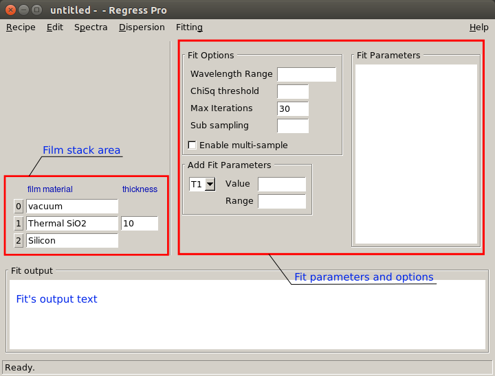
In the figure below you can see the main window of Regress Pro and the area where the film stack is configured with the corresponding thicknesses on the right.
Editing the Film Stack
The recipe’s film stack can be edited directly from the main window. The thickness of a layer can be entered or modified by editing the text field on the right of the film. A button is also present of the left of each layer to perform layer-related operations. By left-clicking on the button close to the layer is possible to add or delete a layer, change the film’s model or modify the model using the edit function. In the bottom part of the menu it is possible also to save the film into the user’s library, save it into a file or plot the dispersion curve.
The user’s library is a list where dispersion model modified by the user can be added. Once a material is addeded in the user’s library it will be available to be used for the whole working session.
Tip
Be careful to save into a file the dispersions you need for later use. When the application is closed all the models in the user’s library are lost.
Loading a Spectrum
To work with Regress Pro one usually load an experimental spectrum to be analyzed. The applications accept a variery of spectroscopic spectra from ellipsometers or reflectometers. To load a spectrum use the menu function “Spectra -> Load Spectra” and choose the file. Once the file is loaded it can visualized it by using the interactive fit window.
The interactive fit window can be opened using the menu function “Fitting -> Interactive Fit”. In this window you can experiment interactively with your data on the base of the defined Result Stack. Please note that the Result Stack is not the same of the film stack found into the main window. The result stack can be accessed using the menu function “Fitting -> Edit Result Stack”. More details about the result stack are given later.
For the moment we focus on the recipe’s film stack shown on the main window. In the next section we explain how to setup a film stack and define a fit recipe.
Fit Recipe
A fit recipe is defined by a list of fitting parameters each with a corresponding seed value and an optional range. The fit parameters are configured in the main window in the area shown in the figure above. The entries are chosen from the list and added with the “return” key. When adding a parameter a seed value can be explicitly given or otherwise the seed will be marked an undefined. When the seed value is undefined its nominal value will be retrieved from the film stack.
When entering a seed value a range can be also optionally given. If a range is given the system will perform a grid search for the given parameter around the seed value plus and minus the range. The step size for the grid search is automatically determined by the application. The grid search is an useful option to ensure that the non-linear fit algorithm can found a global, optimal, solution.
Note
If the grid search is made on multiple parameters the search space can be very large and the grid search can take a very long time. When you need to specify a range try to use it only for a very small number of parameters, ideally not more than three.
Fit Parameters
The list of the available fit parameters depends on the film stack. For any given stack the thicknesses of each film will be available in the parameters list. The thicknesses are are named T1, T2, T3, ... where T1 is the top layer, T2 is the layer below and so on and their values are always expressed in Angstrom.
When a film stack use a dispersion model for any of the layers the corresponding parameters will be available in the parameters list. The model parameters are grouped by layer number and named accordingly to the model.
Adding a model parameters means that the fit will adjust its value to find an optimal solution.
For any fitting parameter, thickness or model parameter, you can specify a seed value to be used as a starting point and you can optionally give a range.
Note
A range for model parameters is only needed if the corresponding range to explore is such that the model’s behavior is strongly not linear. Try to avoid specifying a range if it is not strictly needed as this can lead to a very time-consuming search in the parameters’s space.
Running the Fit Recipe
Once the film stack is configured and the list of fit parameters is defined with the corresponding seed values the fit can be done using th menu function “Fitting -> Run Fitting”. When the fit terminate the results will be shown in the bottom part of the main windows.
The output will include the optimized value of each parameter and the residual Chi Square.
Note
The fit is done using the Levenberg–Marquardt non-linear fit algorithm. It is a method that finds a solution that minimise the sum of squares of the residual between the experimental data and the model. If a range is specified for one or more parameters a grid search is done before the Levenberg–Marquardt minimization. The search works looking to the residuals and choose the point in the grid with the smaller residuals. The point selected by the grid search is used as the initial seed for the Levenberg–Marquardt non-linear fit.
Once the fit is terminated you can visualize the experimental data together with the theoretical curve by opening the interactive fit window. This latter can be opened using the menu function “Fitting -> Interactive Fit”.
It is important to know that when you perform a fit:
- the “Result Stack” is updated with fit’s result values
- the interactive fit is updated also accordingly to the fit’s results.
The “Result Stack” is a film stack where the results of the fit are stored. On the other side, the film stack shown in the main window is not modified when you run a fit. So, in general, if you want to inspect the results of the fit you should look to the “Result Stack”. This latter is accessible using the menu function “Fitting -> Edit Result Stack”.
Interactive Fit Window
In the previous section we said that the interactive fit window is modified according to the fit’s results. While this is true, in reality the general rule is that the interactive fit window is directly linked to the “Result Stack”. This means that any change made on the “Result Stack” will be reflected in the interactive fit and viceversa. You can also edit the result stack and see the changes reported to the interactive fit window.
Note
The fact that the interactive fit window is linked to the result stack means that if you want to change the model used for the interactive fit you need to make the changes in the “Result Stack”. For example you could go in the result stack and change a dispersion model, add a layer or something else and then come back to the interactive fit window. Just be aware that when you run the fit recipe from the main window the result stack will be overwritten so be careful to save any important elements before running a fit recipe.
Running an Interactive Fit
The interactive fit is a window that shows the experimental spectrum, in red, along with the theoretical spectrum, in blue. The theoretical spectrum will be calculated on the basis of the result stack. On the left side of the window it is shown the list of all the possible fit parameters along with their corresponding values.
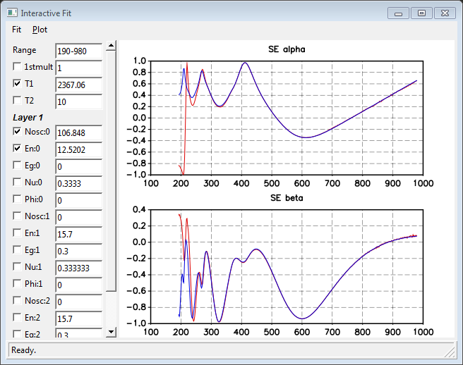
The interactive fit window let you change the value of any parameters directly by typing the value on the text entry. When a value is changed the result will be immediately reflected by the theoretical spectrum. It is also possible to perform a fit by checking the desired parameters and using the menu function “Fit -> Run”.
It is also possible to change the spectral range of the data by using the “Range” entry. The interval should be given in the form “200-800” with the two wavelength limits in nanometers separated by a “-” (minus). Changing the spectra range will affect the visualization but also the data actually used of the fit.
The interactive fit is very useful because it let you experiment to see how the ellipsometry or reflectometry response changes with each of the parameters. The value of each parameter can be changed to see how the response changes and verify when the model response get close to the experimental spectrum.
Tip
You can undo and redo any operations in the fit window by using the corresponding menu functions or the shortcuts “Control-Z” and “Control-R”. The undo operation can be very useful if you mess up a complicated setup and you want to come back to a previous set of values.
Tip
It is possible to change the value of a parameter by positioning the cursor and pressing the key combinations “Shift-Up” or “Shift-Down”. Using this shortcut will increase or decrease the value for the digit on the left of the cursor. This is very handy to rapidly check how a parameter affect the spectrum without having to type the whole number each time. By positioning the cursor you can also choose to modify the parameter by a small amount of by a big amount, depending on the digit you chose.