Fast Fourier Transform
Mathematical Definitions
Fast Fourier Transforms are efficient algorithms for calculating the discrete Fourier transform (DFT)
The DFT usually arises as an approximation to the continuous Fourier
transform when functions are sampled at discrete intervals in space or
time. The naive evaluation of the discrete Fourier transform is a matrix-vector multiplication  . A general matrix-vector multiplication takes O(n2) operations for n data-points. Fast Fourier transform algorithms use a divide-and-conquer strategy to factorize the matrix W into smaller sub-matrices, corresponding to the integer factors of the length n. If n can be factorized into a product of integers f1 f2 … fm then the DFT can be computed in O(n Σ fi) operations. For a radix-2 FFT this gives an operation count of O(n log2 n).
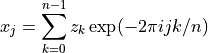
All the FFT functions offer two types of transform: forwards and inverse, based on the same mathematical definitions. The definition of the forward Fourier transform, fft(z), is,
and the definition of the inverse Fourier transform is,
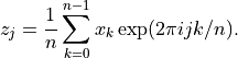
The factor of 1/n makes this a true inverse.
In general there are two possible choices for the sign of the exponential in the transform/ inverse-transform pair. GSL follows the same convention as fftpack, using a negative exponential for the forward transform. The advantage of this convention is that the inverse transform recreates the original function with simple Fourier synthesis. Numerical Recipes uses the opposite convention, a positive exponential in the forward transform.
GSL Shell interface
GSL Shell provide a simple interface to perform Fourier transforms of real data with the functions num.fft() and num.fftinv().
The first function performs the Fourier transform of a column matrix and the second is the inverse Fourier transform.
The function num.fft() returns a half-complex array.
This latter is similar to a column matrix of complex numbers, but it is actually a different object because the numbers are packed together following some specific rules related to the algorithm.
The idea is that you can access the elements of this vector for reading or writing simply by indexing it.
You can also obtain the size of the vector using the operator ‘#’.
The valid indices for a half-complex object range from 0 to N-1 where N is the size if the vector.
Each element of the vector corresponds to the coefficient  defined above.
When performing Fourier transforms, it is important to know that the computation speed can be greatly influenced by the size of the vector. If the size is a power of two, a very efficient algorithm can be used and we can talk in this case of a Fast Fourier Transform (FFT). In addition, the algorithm has the advantage that it does not require any additional workspace. When the size of the vector is not a power of two, we can have two different cases:
the size is a product of small prime numbers
the size contains a big (> 7) prime number in its factorization
This detail is important because if the size is a product of small prime numbers, a fast algorithm is still available but it is still somewhat slower and it does require some additional workspace. In the worst case when the size cannot be factorized to small prime numbers, the Fourier transform can still be computed but the calculation is slower, especially for large arrays.
GSL Shell hides all the details and takes care of choosing the appropriate algorithm based on the size of the vector. It also transparently provides any additional workspace that may be needed for the algorithm. In order to avoid repeated allocation of workspace memory, the workspace allocated is kept in memory and reused if the size of the array does not change. This means that the approach of GSL Shell is quite optimal if you perform many Fourier transforms (direct or inverse) of the same size.
Even though GSL Shell takes care of the details automatically, you should be aware of these performance notices because it can make a big difference in real applications. From a practical point of view, it is useful in most cases to always provide samples whose size is a power of two.
Another property of the functions num.fft() and num.fftinv() is that they can optionally perform the transformation in place by modifying the original data instead of creating a copy.
When a transformation in place is requested, the routine still returns a new vector (either a real matrix or a half-complex array) but this latter will point to the same underlying data of the original vector.
The transformation in place can be useful in some cases to avoid unnecessary data copying and memory allocation.
Fourier Transform of Real Data
For real data, the Fourier coefficients satisfy the relation

where N is the size of the vector and k is any integer number from 0 to N-1. Because of this relation, the data is packed in a special type of object called a half-complex array.
To access an element in a half-complex array, you can index it with an integer number between 0 and N-1, inclusive. So, for example:
-- get a random number generator
r = rng.new()

-- create a vector with random numbers
x = matrix.new(256, 1, || rnd.gaussian(r, 1))

-- take the Fourier transform
ft = num.fft(x)

-- print all the coefficients of the Fourier transform
for k=0, #ft-1 do print(ft[k]) end
As shown in the example above, you can use the Lua operator ‘#’ to obtain the size of a half-complex array.
- num.fft(v[, in_place])
Perform the Fourier transform of the real-valued column matrix
x. Ifin_placeistruethen the original data is altered and the resulting vector will point to the same underlying data of the original vector.Please note that the value you obtain is not an ordinary matrix but a half-complex array. You can access the elements of such an array by indexing the vector. If you want to have an ordinary matrix you can easily build it with the following instructions:
-- we suppose that f is an half-complex array
m = matrix.cnew(#f, 1, |i,j| f[i-1])
- num.fftinv(hc[, in_place])
Return a column matrix that contains the inverse Fourier transform of the half-complex vector
hc. Ifin_placeistruethen the original data is altered and the resulting vector will point to the same underlying data of the original vector.This transformation is the inverse of the function
num.fft(), so that if you perform the two transformations consecutively you will obtain a vector identical to the initial one.A typical usage of
fft_inv()is to revert the transformation made withfft()but by doing some transformations along the way. So a typical usage path could be:-- we assume v is a column matrix with our data ft = num.fft(v) -- Fourier transform -- here we can manipulate the half-complex array 'ft' -- using the methods `get' and `set' some code here vt = num.fftinv(ft) -- we perform the inverse Fourier transform -- now vt is a vector of the same size of v
FFT example
In this example we will treat a square pulse in the temporal domain. To illustrate a typical example of FFT usage we perform the Fourier Transform of the signal and we cut the higher order frequencies. Then we perform the inverse transform and we compare the result with the original time signal.
So, first we define our square pulse in the time domain. Actually it will be a matrix with just one column:
n, ncut = 256, 16

-- we create a pulse signal in the time domain
y = matrix.new(n, 1, |i| i < n/3 and 0 or (i < 2*n/3 and 1 or 0))
Then we create two new plots, one for the Fourier transform and one for the signal itself:
pt = graph.plot('Original signal / reconstructed')

pt:addline(graph.filine(|i| y[i], 1, n), 'black')
Now we are ready to perform:
the Fourier transform
cut the higher frequencies
transform back the signal in the time domain
and plot the results:
ft = num.fft(y)

pf = graph.fibars(|k| complex.abs(ft[k]), 0, 60)
pf.title = 'FFT Power Spectrum'

for k=ncut, n/2 do ft[k] = 0 end
ytr = num.fftinv(ft)

pt:addline(graph.filine(|i| ytr[i], n), 'red')

pt:show()
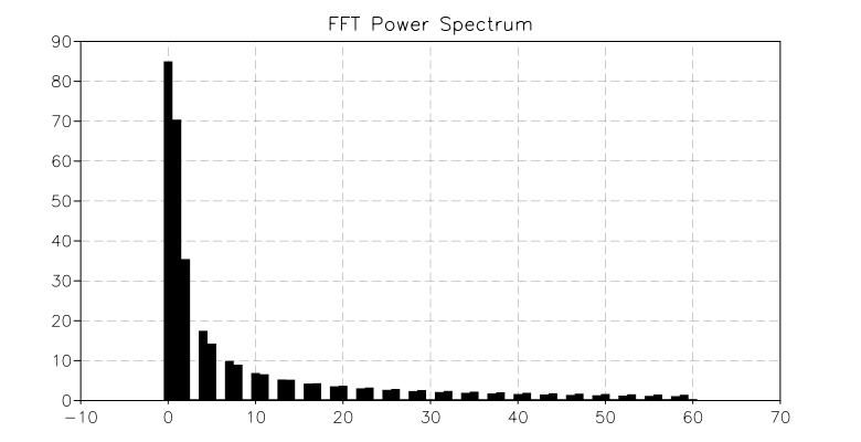
Fourier transform spectrum
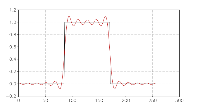
Time signal before (black) and after (red) the transformation
You can observe in the reconstructed signal (the red curve) that we obtain approximately the square pulse, but with a lot of oscillations. Of course this is an artifact of our transformations. The reason is that in order to perfectly reproduce a sharp signal, we also need all the high frequencies of the Fourier transform.