Contour Plots

Overview

GSL shell offers a contour plot function to draw contour curves of bidimensional functions. The current algorithm works correctly only for continuous functions and it may give bad results if the function has discontinuities.

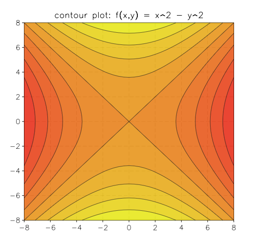
Here is an example of its utilization to plot the function \(f(x,y) = x^2 - y^2\):

contour.plot(function(x,y) return x^2 - y^2 end, -8, -8, 8, 8)

contour.plot(f, xmin, ymin, xmax, ymax[, options])

Plot a contour plot of the function f in the rectangle delimited by (xmin, ymin), (xmax, ymax) and return the plot itself.

The options argument is an optional table that can contain the following fields:

• gridx, number of subdivision along x
• gridy, number of subdivision along y
• levels, number of contour levels or a list of the level values in monotonic order.
• colormap a function that returns a color for the contour region. The argument of the function will be a number between 0 and 1.
• show, specify if the plot should be shown. By default it is true.

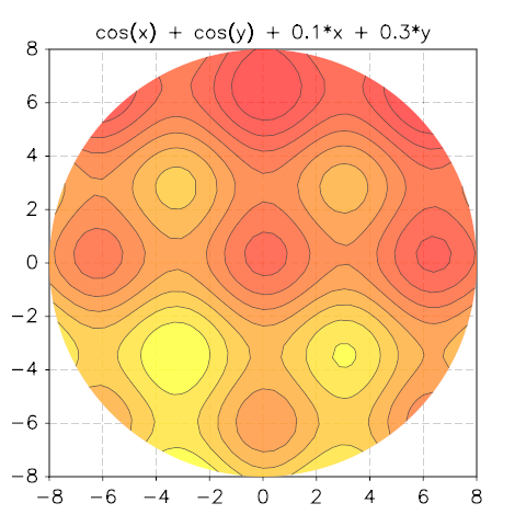
contour.polar_plot(f, R[, options]])

Plot a contour plot of the function f(x, y) over the circular domain of radius R and centered at the origin. The options table accepts the same fields as the function contour().

Example:

use 'math'

p = contour.polar_plot(function(x,y) return cos(x)+cos(y)+0.1*x+0.3*y end, 8)
p.title = 'cos(x) + cos(y) + 0.1*x + 0.3*y'